Getting our hands dirty with beta functions

We just finished watching a YouTube tutorial on Dirichlet distributions given by Foursquare data scientist Max Sklar. According to Wikipedia, the Dirichlet distribution is the “multivariate generalization of the beta distribution.” Yikes! We confess that the last time we saw a beta distribution was around the time Bill Clinton was being impeached. In this post we brush the cobwebs from our minds and derive a basic identity between beta and gamma functions and illustrate our calculations with R.

Beta distributions are defined by density functions

$$f(x; \alpha, \beta) = \frac{1}{B(\alpha, \beta)} x^{\alpha - 1} (1 - x)^{\beta - 1},$$

where $\alpha$ and $\beta$ are shape parameters and $B$ is the beta function defined as:

$$\begin{align} B(\alpha, \beta) &:= \int_0^1 t^{\alpha - 1}(1 - t)^{\beta - 1} dt \\ &= \frac{\Gamma(\alpha)\Gamma(\beta)}{\Gamma(\alpha + \beta)}\label{eq:one} \end{align}$$

The definition of $B(\alpha, \beta)$ above reflects the fact that $f$ is a probability density function and must integrate to 1. Rather infuriatingly, Wikipedia states that the second line simply “follows from the definition of the gamma function” without any further explanation. We derive this identity below.

Let $U$ and $V$ be independent random variables with gamma distributions

$$\begin{align} U &\sim \frac{1}{\Gamma(\alpha)} u^{\alpha - 1} e^{-u} & V &\sim \frac{1}{\Gamma(\beta)} v^{\beta - 1} e^{-v}. \end{align}$$

We transform $U$ and $V$ to random variables $X$ and $Y$ using the equations

$$\begin{align} X &= \frac{U}{U + V} & Y &=U + V \\ U &= XY & V &= Y - XY \end{align}$$

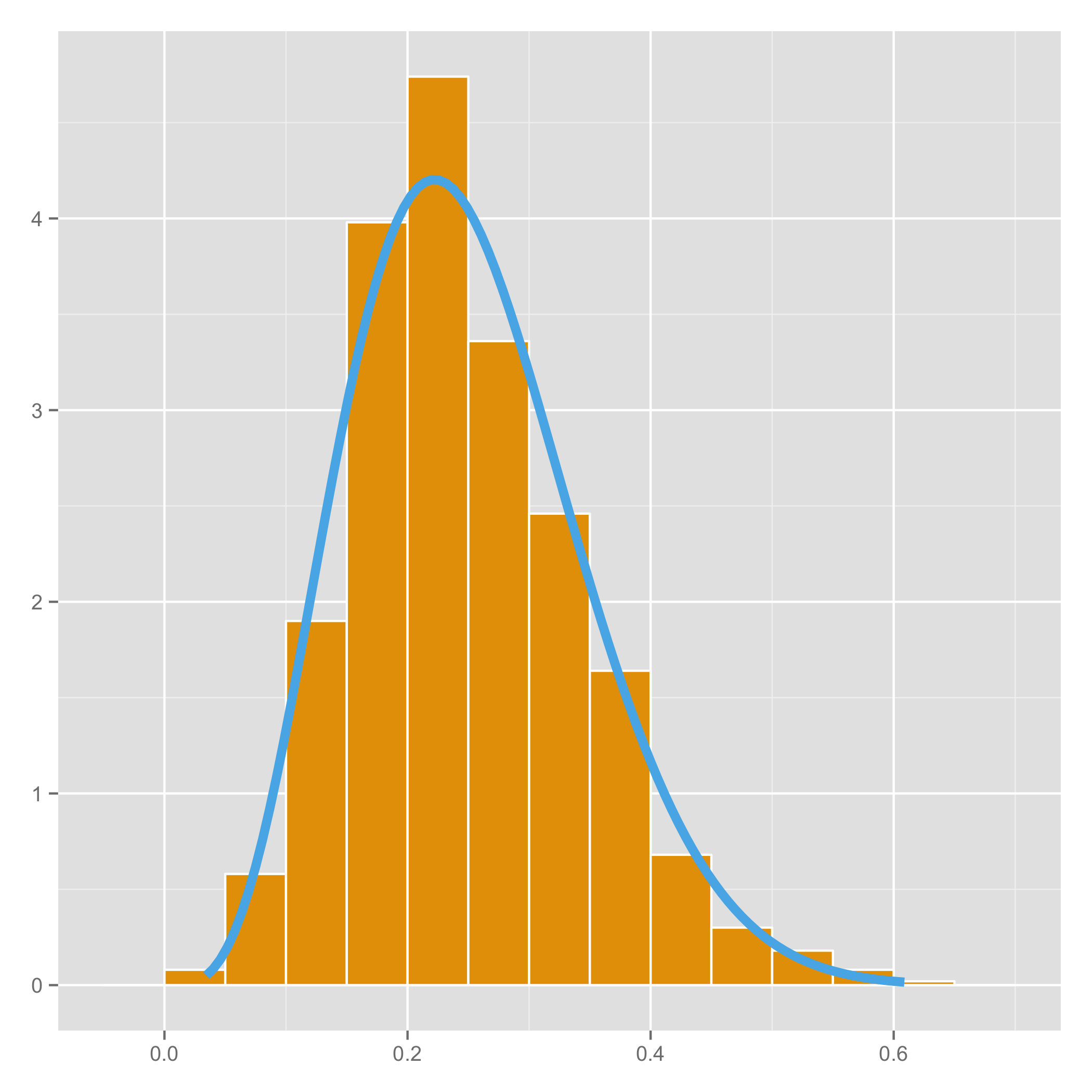
Here comes a wonderful fact: the pdf of $X$ is a beta distribution. Before we prove this, we visualize it with some R code:

library(ggplot2)
# change these parameters if you want
alpha <- 5
beta <- 15
nSamples <- 1000
# generate samples for U and V according to gamma distributions with shape alpha and beta
u <- rgamma(1000, shape = alpha)
v <- rgamma(1000, shape = beta)
# transform the variables to x and y
x <- u / (u + v)
y <- u + v
# data for pdf of the beta function with shapes alpha and beta
xBeta <- seq(min(x), max(x), length = 100)
yBeta <- dbeta(xBeta, shape1 = alpha, shape2 = beta)
# plot the density of x versus the pdf of the beta distribution
myPlot <- ggplot() +
    geom_histogram(aes(x, y = ..density..),
                   binwidth = 0.05,
                   color = "white",
                   fill = "#E69F00") +
    geom_line(aes(x = xBeta, y = yBeta), color = "#56B4E9") +
    theme(axis.title.x = element_blank()) +
    theme(axis.title.y = element_blank())
# ...profit!
plot(myPlot)

This code generates the pretty picture at the top of this article. The orange bars are a histogram for 1000 random samples of $X$, and the blue line represents the graph of beta distribution $f(x;\alpha,\beta)$. You can see that the blue line matches up nicely with the orange bars.

On to the business of showing our identity. Since $U$ and $V$ are independent, the joint distribution of $(U,V)$ is

$$f(u,v) = \frac{1}{\Gamma(\alpha)\Gamma(\beta)} u^{\alpha - 1} v^{\beta - 1} e^{-u - v}.$$

The Jacobian of the transformation $(X,Y) \mapsto (U,V)$ is

$$\begin{vmatrix} \frac{\partial{u}}{\partial{x}} &\frac{\partial{u}}{\partial{y}} \\ \frac{\partial{v}}{\partial{x}} &\frac{\partial{v}}{\partial{y}} \end{vmatrix} = \begin{vmatrix}y & x \\ -y & 1 - x \end{vmatrix} = y.$$

The joint distribution of $(X,Y)$ is thus

$$\begin{align} g(x,y) &= f(xy, y - xy) y \\ &=\frac{1}{\Gamma(\alpha)\Gamma(\beta)}(xy)^{\alpha - 1}(y - xy)^{\beta - 1} y e^{-y} \\ &=\frac{1}{\Gamma(\alpha)\Gamma(\beta)}x^{\alpha - 1}(1 - x)^{\beta - 1} y^{\alpha +\beta - 1} e^{-y} \end{align}$$

and the pdf of $X$ is found by integrating along the $y$ values of this equation.

$$\begin{align} f(x)&= \frac{1}{\Gamma(\alpha)\Gamma(\beta)} x^{\alpha - 1}(1 - x)^{\beta - 1} \int_0^\infty y^{\alpha + \beta - 1} e^{-y} dy \\ &= \frac{\Gamma(\alpha + \beta)}{\Gamma(\alpha)\Gamma(\beta)} x^{\alpha - 1}(1 - x)^{\beta - 1} \end{align}$$

Our identity follows from the fact that $f(x)$ is a pdf and must integrate to 1.

$$\begin{align} 1 &= \int_0^1 \frac{\Gamma(\alpha + \beta)}{\Gamma(\alpha)\Gamma(\beta)} t^{\alpha - 1}(1 - t)^{\beta - 1} dt \\ \frac{\Gamma(\alpha)\Gamma(\beta)}{\Gamma(\alpha + \beta)} &= \int_0^1 t^{\alpha - 1}(1 - t)^{\beta - 1} dt \end{align}$$

Conclusion

This was a nice little exercise to help us remember some statistics.

---

---

blog comments powered by Disqus

Written by

Stephanie Yang

Published

Tags

• stephanie 5
• statistics 4